Note
Go to the end to download the full example code.
Multislice 2D to 3D translation (T2*)#
This example illustrates 2D to 3D coregistration using 3D translations
The moving volume is an oblique multi-slice T2* map and the static volume is a 3D coronal mask covering both kidneys.
An initial 3D translation is performed using both kidneys as a static target. In a second step, fine tuning is done for each kidney separately.
Coregistration is performed by brute force optimization using a mutual information metric.
Setup#
# Import packages
import vreg
import vreg.plot as plt


# Get static volumes
lk = vreg.fetch('left_kidney')
rk = vreg.fetch('right_kidney')

# get moving volumes
multislice = vreg.fetch('T2star')

# Get geometrical reference
dixon = vreg.fetch('Dixon_water')
Format data#
Create a mask containing both kidneys (bk) with the geometry of the complete DIXON series
bk = lk.slice_like(dixon).add(rk)
Extract bounding boxes to reduce the size of the volume. This is not necessary but it speeds up the calculation a little as the volume is smaller.
bk = bk.bounding_box()
lk = lk.bounding_box()
rk = rk.bounding_box()
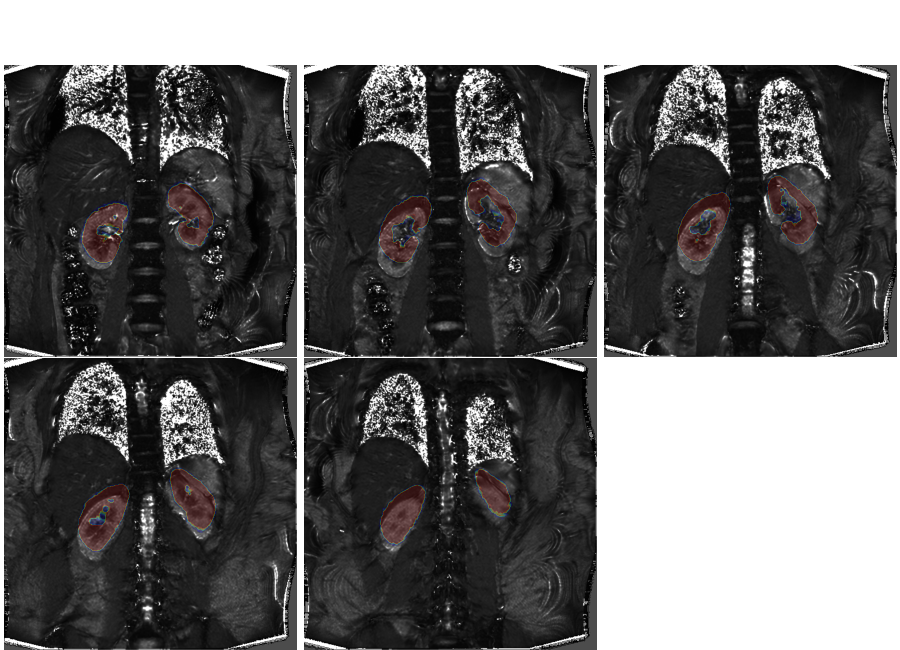
If we overlay the mask on the volume, we clearly see the misalignment due to different breath holding positions:
plt.overlay_2d(multislice, bk)

Coregister to both kidneys#
In a first step we coregister by 3D translation to both kidneys. Since the moving data are multislice, we need to perform a coregistration for each slice separately. We perform brute force optimization allowing translations between [-20, 20] mm in-slice, and [-5, 5] mm through-slice, in steps of 2mm:
# Optimizer settings
optimizer = {
    'method': 'brute',
    'grid': (
        [-20, 20, 20],
        [-20, 20, 20],
        [-5, 5, 5],
    ),
}
# Translations are defined in volume coordinates
options = {
    'coords':'volume',
}
# Perform the coregistration for each slice
for z, sz in enumerate(multislice):
    tz = sz.find_translate_to(bk, optimizer=optimizer, **options)
    multislice[z] = sz.translate(tz, **options)
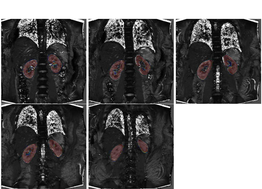
If we overlay the mask on the new volume, we can see that the misalignment is significantly reduced but some imperfections still remain.
plt.overlay_2d(multislice, bk)

Left kidney fine tuning#
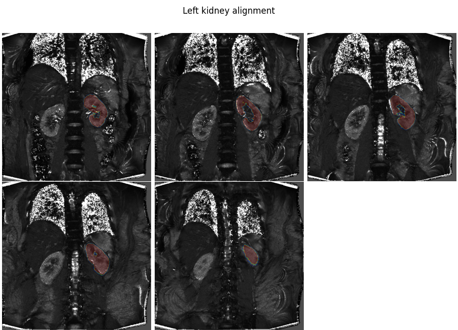
We now perform a rigid transformation to the left kidney to fine tune the alignment.
Plot the result
plt.overlay_2d(align_lk, lk, title='Left kidney alignment')

Right kidney fine tuning#
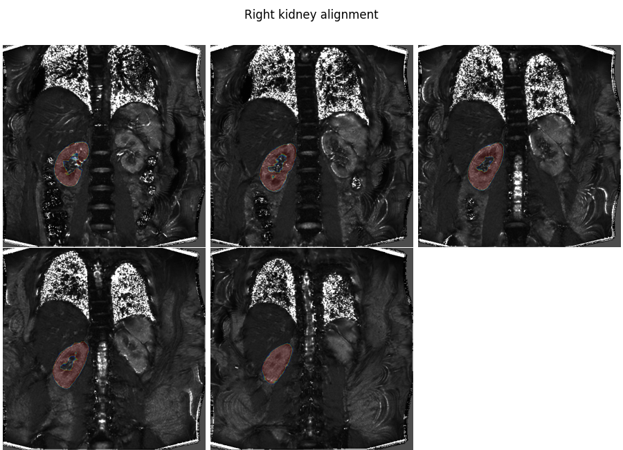
Repeat the same steps for the right kidney
Plot the result
plt.overlay_2d(align_rk, rk, title='Right kidney alignment')

Total running time of the script: (22 minutes 39.181 seconds)